Machine Learning Workflow Explained Visually: From Data to Deployment
If you are stepping into the world of Artificial Intelligence, you have likely spent hours reading about neural networks, decision trees, and optimization algorithms. But here is an industry secret that surprises many beginners:
Writing the algorithm is only about 10% of the actual job.
In the real world, a model living inside a local Jupyter Notebook is virtually useless. To deliver actual business value, that mathematical model must be integrated into a structured, resilient machine learning workflow. A model that performs perfectly in training but fails in production is worse than useless — it is misleading.
Many self-taught learners struggle because they focus solely on the math, entirely missing the broader machine learning process. Understanding the end-to-end machine learning workflow — how data is gathered, cleaned, transformed, evaluated, and deployed into a live environment — is exactly what separates a beginner from a production-ready ML engineer.
In this guide, we are going to explore the machine learning workflow explained visually. We will break down every stage of the ML lifecycle, look at real-world production scenarios, and give you interactive ways to build your ML intuition.
1. High-Level Machine Learning Workflow Overview
What Is a Machine Learning Workflow?
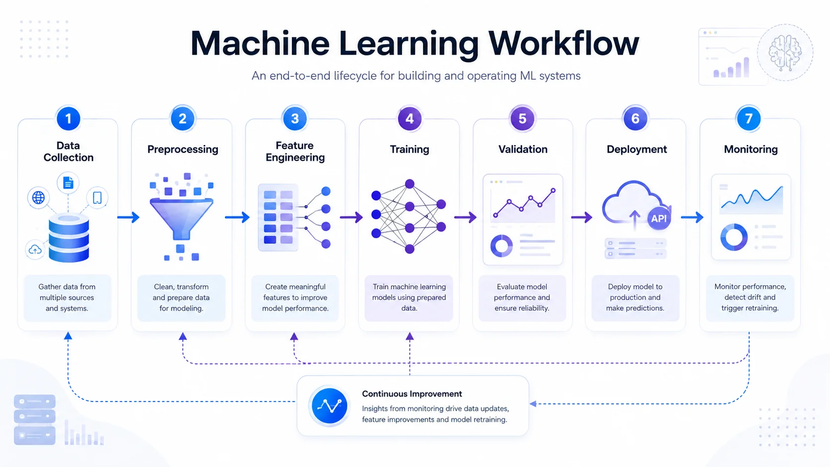
A machine learning workflow is the end-to-end infrastructure used to design, create, and deploy an ML model. It consists of seven stages: data collection, preprocessing, feature engineering, model training, validation, deployment, and continuous monitoring. This pipeline ensures models remain accurate in real-world production environments.
Think of it as a continuous loop, not a straight line. Here are the 7 core stages of a standard machine learning architecture:
- Data Collection: Gathering the raw materials required for the task.
- Data Preprocessing: Cleaning and organizing the chaotic raw data.
- Feature Engineering: Transforming data into clear signals that help algorithms learn.
- Model Training: Feeding the prepared data into an algorithm to recognise patterns.
- Validation & Evaluation: Testing the model against unseen data to prove it works.
- Deployment: Pushing the model to a live production environment.
- Monitoring & Iteration: Watching the model's real-world performance and updating it continuously.
Imagine building a smart factory. Data collection is mining the raw materials. Preprocessing refines them. Model training is the assembly line. Deployment is shipping the product, and monitoring is quality assurance. Good ML workflows optimise for reliability, not just accuracy.
2. Data Collection: The Foundation of the ML Lifecycle
Every machine learning pipeline begins with data. The quality, quantity, and relevance of the data you collect dictate the absolute ceiling of your model's potential.
Where Does Data Come From?
Data can be structured (neatly organized in rows and columns) or unstructured (messy and complex, like images, audio, or text). Common sources include:
- Relational Databases: SQL databases containing user profiles or financial logs.
- APIs: Pulling live weather data, stock prices, or social media metrics.
- Sensors and IoT: Gathering machine-health metrics in real-time.
- User Interactions: Tracking clicks and scroll depth in an app.
Imagine training a resume-screening AI strictly on historical hiring data from a company that previously only hired from one specific university. What happens? The model becomes inherently biased, favouring that university and unfairly rejecting others. Data collection is where bias begins.
Why this matters in production: If a production model is fed stale or unrepresentative data, it will confidently make terrible decisions at scale.
3. Data Preprocessing: Cleaning the Mess
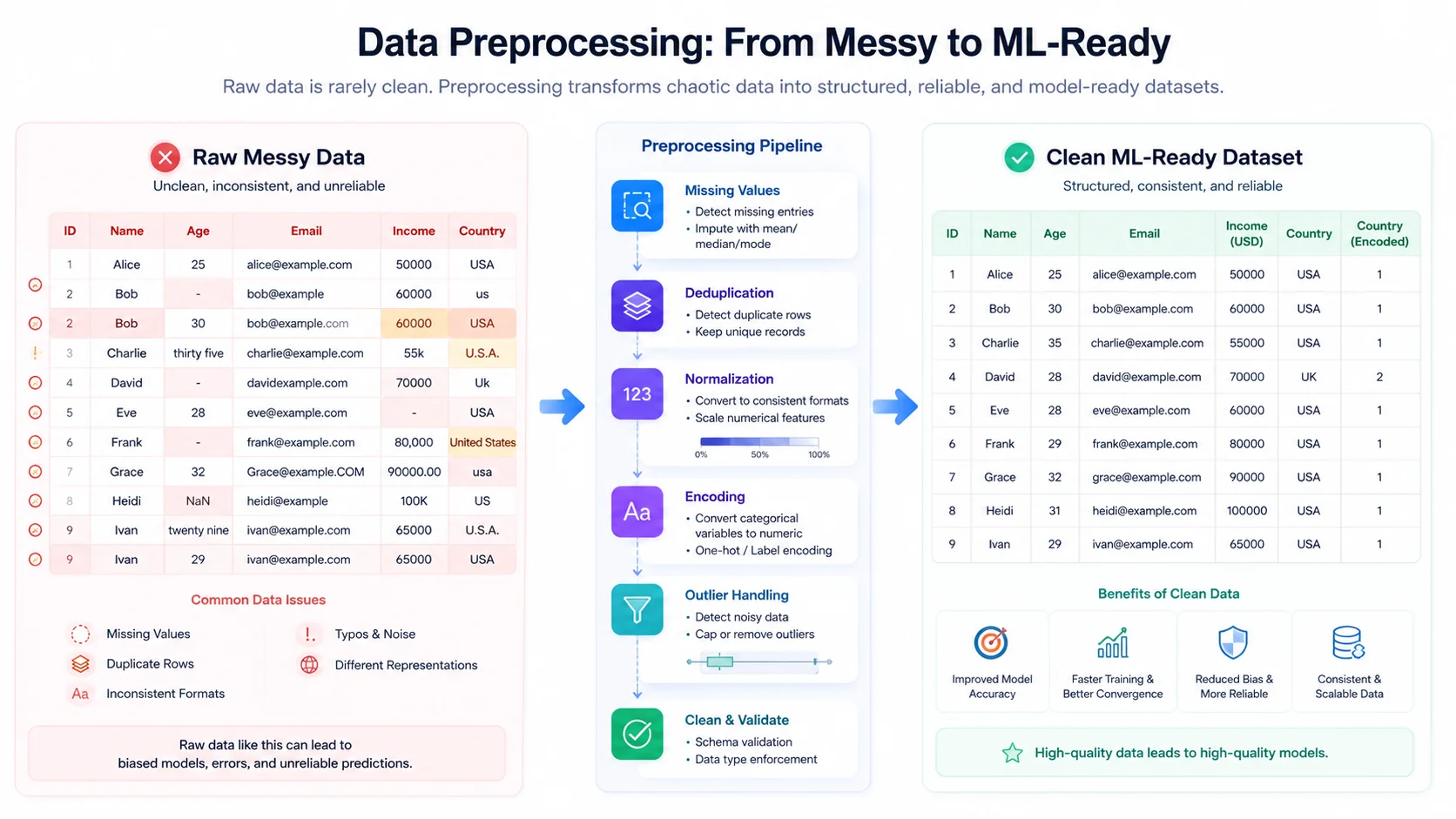
Real-world data is chaotic. It has missing values, duplicate entries, bizarre outliers, and formatting errors. Visualise thousands of rows of customer data where half the phone numbers are missing, and dates are formatted in three different ways.
Data preprocessing is the act of turning this chaos into a structured format that a machine can actually digest. This stage often consumes up to 60% of a data scientist's time.
Essential Preprocessing Techniques
| Preprocessing Technique | What It Means | Practical Example |
|---|---|---|
| Handling Missing Values | Dealing with blank cells in your dataset. | Replacing a missing "Age" value with the median age of all users. |
| Deduplication | Removing identical rows. | Deleting a double-submitted form entry from a database. |
| Categorical Encoding | Turning text labels into numbers. | Converting "Red, Green, Blue" into 0, 1, 2. |
| Outlier Removal | Dropping mathematically absurd data. | Removing a house price listed at $10 because of a typo. |
The Train-Test Split
One of the most critical preprocessing steps in the model training workflow is splitting your data. You cannot test your model on the same data you used to train it.
- Training Set (70–80%): Used to teach the model.
- Testing Set (20–30%): Hidden from the model during training, used strictly for final evaluation.
Data Leakage occurs when information from the test set accidentally leaks into the training set. The model will look incredibly accurate during development but will fail completely the second it is deployed into production.
By this stage, you should understand that raw data is unusable. You must clean it, handle missing values, and strictly separate your training data from your testing data to prevent artificial accuracy.
4. Feature Engineering: Crafting the Right Signals
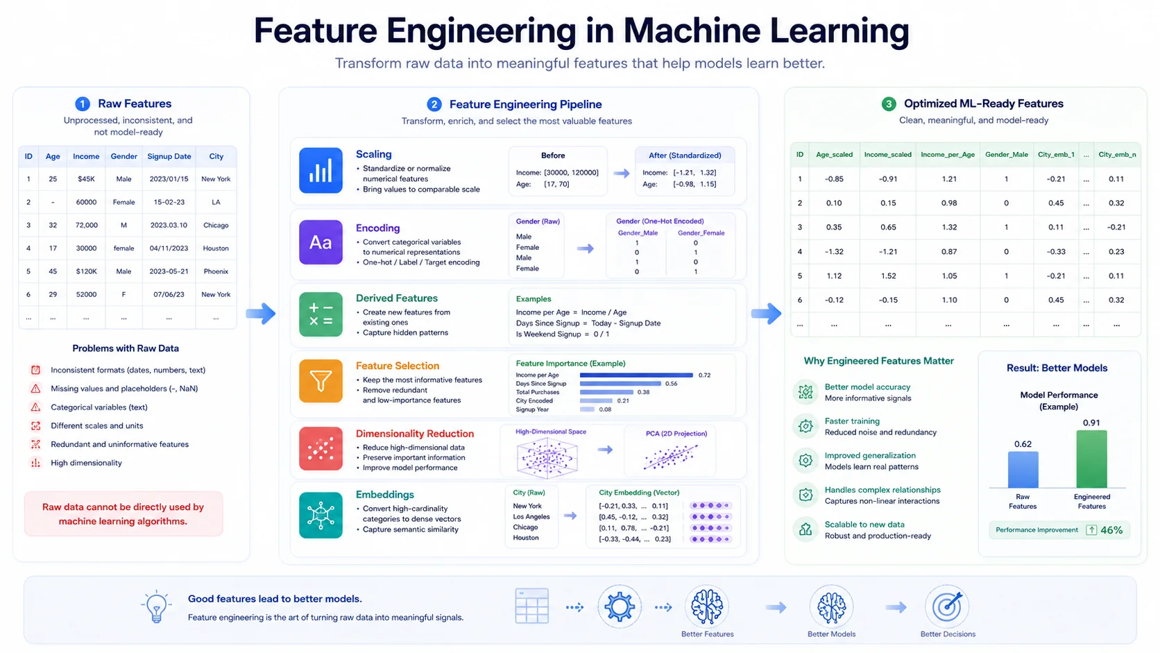
If preprocessing is about cleaning the data, feature engineering is about enhancing it. A "feature" is simply an input variable (a column in your dataset).
Algorithms learn, but features teach. Sometimes, the raw data isn't in the best format for an algorithm to find patterns. Feature engineering involves creating new features, selecting the best ones, and scaling them.
Advanced Feature Engineering Concepts
- Derived Features: Combining data to make it more useful. An algorithm might struggle to use a "Date of Birth" column, but if you engineer a new column called "Age," it instantly understands the value.
- Feature Scaling: Algorithms get confused by different scales. Scaling shrinks all features into a uniform range (like 0 to 1) so a $200,000 income doesn't mathematically overpower a 35-year age.
- Dimensionality Reduction: Techniques like PCA (Principal Component Analysis) help reduce thousands of features down to the most important ones, preventing the model from becoming slow and confused.
Embeddings are the ultimate feature engineering for modern AI. They convert words, sentences, or images into dense mathematical vectors so Large Language Models (LLMs) can understand semantic context — the same technique that powers ChatGPT and every modern NLP system.
5. Model Training: Where the Machine Learns
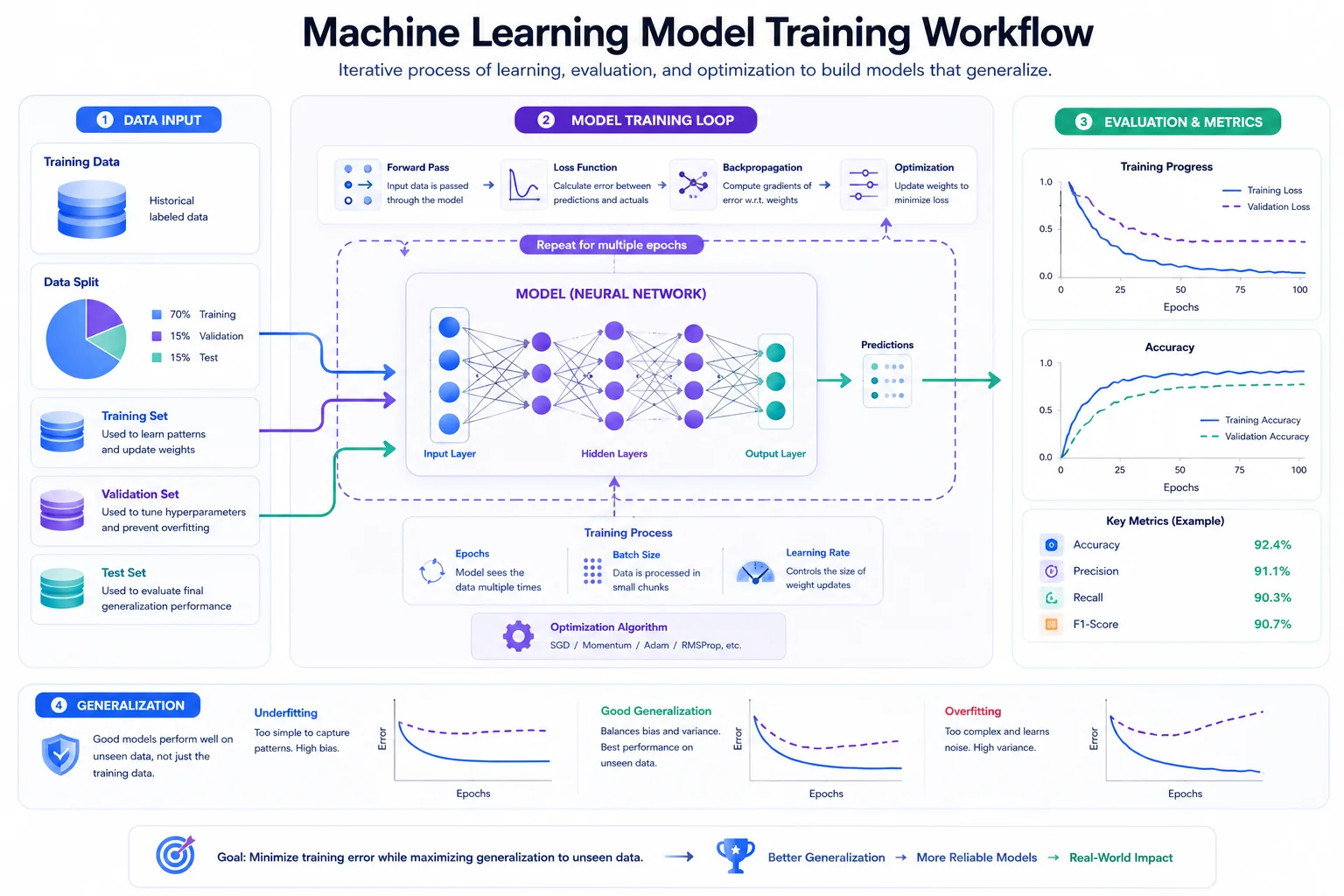
Now that our data is clean and highly optimised, we enter the core model training workflow. This is where the machine finally "learns" using algorithms like Random Forest (great for tabular data) or Neural Networks (great for images and text).
During training, the data is passed through the algorithm in cycles. With each pass, the model makes predictions, calculates how wrong it was, and updates its internal parameters to be slightly more accurate the next time.
The Battle of Generalisation
As the model trains, you must monitor it for two major pitfalls:
| State | What Is Happening? | Real-World Analogy |
|---|---|---|
| Overfitting | The model memorised the training data perfectly but fails on new data. It learned the noise, not the pattern. | A student who memorises a practice test but fails the actual exam. |
| Underfitting | The model is too simple and fails to learn the patterns in the data at all. | A student who barely studies and guesses on every question. |
| Optimal Fit | The model learned the underlying patterns and performs well on unseen data. | A student who understands the core concepts and applies them correctly. |
Before writing complex neural networks, build an intuition for how algorithms react to noisy data. You can generate custom, privacy-safe mock data using the MortalApps Synthetic Dataset Generator. Try creating an intentionally messy dataset and experiment to see exactly how quickly a basic model overfits to the noise.
Training is a balancing act. Your goal is not to get 100% accuracy on the training data. Your goal is to build a model that generalises perfectly to data it has never seen before.
6. Validation & Evaluation: Grading the Model
Once the model is trained, we evaluate it using the testing dataset we hid earlier. Picture a dashboard filling up with metrics — this is where we prove the pipeline actually worked.
Why "Accuracy" Is a Dangerous Metric
Imagine deploying a model into a banking app to detect credit card fraud. Fraud only happens in 0.1% of transactions. If your model simply guesses "Not Fraud" every single time, it will be 99.9% accurate! But it would be entirely useless, costing the bank millions.
Because of this, production ML pipelines rely on deeper evaluation metrics:
- Precision: Out of all predicted positives, how many were actually positive? (Crucial for spam filters — you don't want legitimate emails going to spam.)
- Recall (Sensitivity): Out of all actual positives, how many did the model find? (Crucial for medical diagnoses — you cannot afford to miss a sick patient.)
- F1-Score: The balanced harmonic mean of Precision and Recall.
Evaluating an imbalanced dataset using Accuracy alone can completely hide model failure. Always look at the confusion matrix to see the full picture of true positives, false positives, true negatives, and false negatives.
One of the fastest ways to understand why Accuracy lies is to experiment with different class distributions yourself. You can visualise how false positives and false negatives interact using the interactive MortalApps Confusion Matrix Calculator. Try plugging in a 99% normal / 1% fraud scenario and watch what happens to your Precision and Recall scores when the model makes just a few mistakes.
7. Deployment: Taking the Model Live
You have a highly capable model. Now it needs to be integrated into a software application so users can benefit from it. There are several ways to architect machine learning deployment, depending on business needs:
| Deployment Strategy | How It Works | Best For |
|---|---|---|
| REST APIs / Microservices | The model is hosted on a cloud server. An app sends data to the API, and the API returns the prediction. | Web apps, scalable SaaS products. |
| Batch Inference Pipelines | The model runs periodically on massive databases, not in real-time. | Generating daily "Suggested for You" recommendations. |
| Edge Deployment | The model runs locally on a user's device (smartphone). Zero data leaves the phone. | Privacy-first apps, offline functionality, zero-latency needs. |
Why this matters in production: ML engineers must worry about traditional software concerns. If your API takes 3 seconds to return a prediction, users will abandon the app. Scalable inference and pipeline orchestration are just as important as algorithm choice.
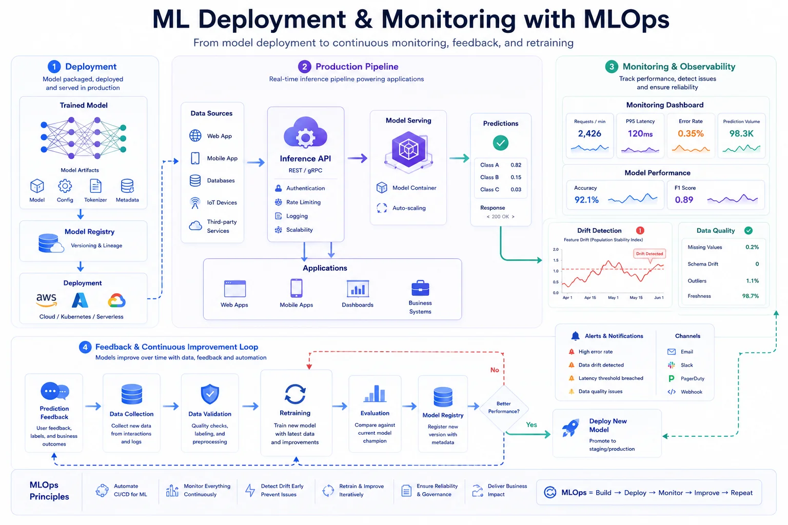
8. Monitoring & Iteration: The Continuous ML Lifecycle
Machine learning is not just about teaching models. It is about maintaining systems.
A major misconception is that once a model is deployed, the job is done. In reality, what happens after deployment is arguably the most complex phase of the entire ML lifecycle. Unlike standard software code, machine learning models degrade over time. The world changes, and user behaviour shifts.
- Data Drift: The incoming real-world data starts looking different from the training data (e.g., a camera sensor gets dirty, permanently changing image inputs).
- Concept Drift: The relationship between the input and output changes (e.g., scammers invent a brand new style of phishing email, rendering old detection rules useless).
To combat drift, teams use MLOps (Machine Learning Operations). Automated dashboards track prediction confidence. When performance drops, an automated feedback loop sends new data back to step one. The model is retrained, validated, and updated continuously.
A model without a monitoring dashboard is a ticking time bomb. Silent production failures — where the model runs without throwing code errors but returns terrible predictions — can cost companies millions before anyone notices.
9. Common Machine Learning Workflow Failures
When building an end-to-end ML workflow, beginners often make architectural mistakes. Here is a cheat sheet of what to avoid:
| Mistake | Real-World Consequence |
|---|---|
| Data Leakage | Fake Accuracy: The model looks perfect in testing but fails completely in production. |
| Ignoring Imbalanced Data | Misleading Evaluation: The model ignores the minority class entirely. |
| No MLOps or Monitoring | Silent Production Failure: The model slowly degrades without triggering any software errors. |
| Inconsistent Preprocessing | Unstable Predictions: The live application formats data differently than the training pipeline. |
| Chasing Algorithm Hype | Wasted Resources: Spending weeks on a Deep Neural Network when a simple decision tree was faster and more explainable. |
10. Real-World Walkthrough: The Spam Filter Pipeline
To cement your understanding, let's visualise how all 7 steps connect in a real-world scenario: Building an Enterprise Spam Filter.
- Data Collection: You pull 100,000 historical emails. Half are marked "Spam," half "Inbox."
- Data Preprocessing: You strip out broken HTML tags, drop duplicate messages, and strictly separate an 80k training set and a 20k test set.
- Feature Engineering: You use NLP embeddings to turn the raw text into mathematical vectors, and engineer a feature that calculates the ratio of uppercase letters.
- Model Training: You feed the 80k processed emails into a Random Forest algorithm.
- Validation & Evaluation: You test on the remaining 20k emails. You optimise heavily for Precision to ensure legitimate work emails never hit the spam folder.
- Deployment: You deploy the model via a scalable REST API microservice. The mail server pings the API, which returns a "Spam" label in under 50 milliseconds.
- Monitoring: Three months later, scammers start using zero-width spaces to bypass the filter (Concept Drift). Your monitoring alerts you. You collect the new spam, retrain the pipeline, and redeploy.
11. Conclusion: The Iterative Nature of ML
The machine learning workflow is a continuous, living system. Moving an ML model from a raw dataset to a robust production environment requires a delicate balance of data engineering, mathematical intuition, and software operations.
While learning algorithms is exciting, mastering the broader pipeline is what makes you a truly capable ML practitioner. Do not just read about these concepts — put them into practice. The best way to build machine learning intuition is to interact with the math yourself, break things on purpose, and visualise the outcomes.
Ready to build your ML intuition? Experiment with the true cost of false positives using the interactive MortalApps Confusion Matrix Calculator, or generate realistic mock data for your next pipeline test with our Synthetic Dataset Generator.
Frequently Asked Questions
A machine learning workflow is the end-to-end infrastructure used to design, create, and deploy an ML model. It consists of seven stages: data collection, preprocessing, feature engineering, model training, validation, deployment, and continuous monitoring. This pipeline ensures models remain accurate in real-world production environments.
The standard ML lifecycle consists of seven sequential stages: Data Collection, Data Preprocessing, Feature Engineering, Model Training, Validation & Evaluation, Model Deployment, and Monitoring & Iteration (MLOps).
Real-world data is chaotic, incomplete, and full of errors. Data preprocessing is critical because machine learning algorithms require structured, clean mathematical input to find patterns. Poor preprocessing directly leads to inaccurate, biased, or broken models.
After a model is trained, it must be evaluated against unseen test data to ensure it can generalise. If it passes evaluation, it is deployed into production (usually via an API) and continuously monitored for data drift and performance degradation.
Models are typically deployed as cloud-based REST APIs or microservices for real-time inference. They can also be deployed via batch inference pipelines (running periodically on large databases) or directly onto edge devices for zero-latency, private predictions.
Model drift is the degradation of a machine learning model's predictive power over time. It occurs because real-world environments constantly change, meaning the historical data used to train the model no longer accurately reflects current reality.