From Prompt to Token: The Complete LLM Inference Pipeline Explained
How modern LLM systems turn a user prompt into a streamed response, and why it is one of the hardest distributed systems problems in production today.
- Eight things happen between hitting Enter and seeing the first token: tokenization, scheduling, prefill, KV cache creation, attention computation, kernel execution, multi-GPU sync, and sampling.
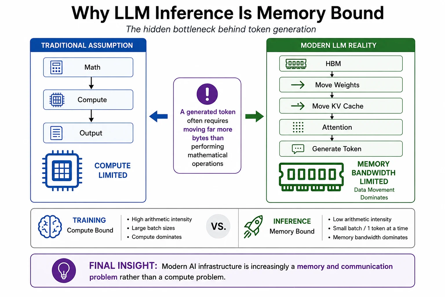
- Generation is not compute-bound: it is memory-bound. The bottleneck is how fast the GPU moves bytes from HBM to its compute cores.
- The KV cache prevents O(N²) recomputation at the cost of GPU memory, the central trade-off of every inference system.
- FlashAttention, GQA, PagedAttention, quantization, and speculative decoding all attack the same constraint: bytes moved per token.
- TTFT (Time To First Token) and TPOT (Time Per Output Token) are optimized differently and require different engineering strategies.
- The LLM Inference Stack at a Glance
- Why Inference Is Harder Than It Looks
- Prompt Arrival: Load Balancing and Continuous Batching
- Tokenization: From Text to Integer IDs
- Prefill vs Decode: The Two Phases of Generation
- Transformer Attention Deep Dive: Q, K, V
- The KV Cache: Why It Exists and What It Costs
- Grouped Query Attention: MHA to GQA
- PagedAttention and Prefix Caching
- The GPU Memory Stack
- HBM: The Real Bottleneck
- Triton and FlashAttention
- TensorRT and Quantization
- Speculative Decoding
- Where Inference Time Actually Goes
- The Four Bottlenecks Framework
- Conclusion
- Frequently Asked Questions
1. The LLM Inference Stack at a Glance
When you send a prompt to an AI model, what actually happens before that first word appears on your screen? To the user, it feels like magic. To a systems engineer, it is a highly orchestrated distributed systems problem constrained by memory bandwidth, interconnect latency, and hardware utilization.
The modern inference stack is not merely about running a neural network forward. It is a pipeline of distinct operational phases, each with its own hardware profile, failure mode, and optimization surface.
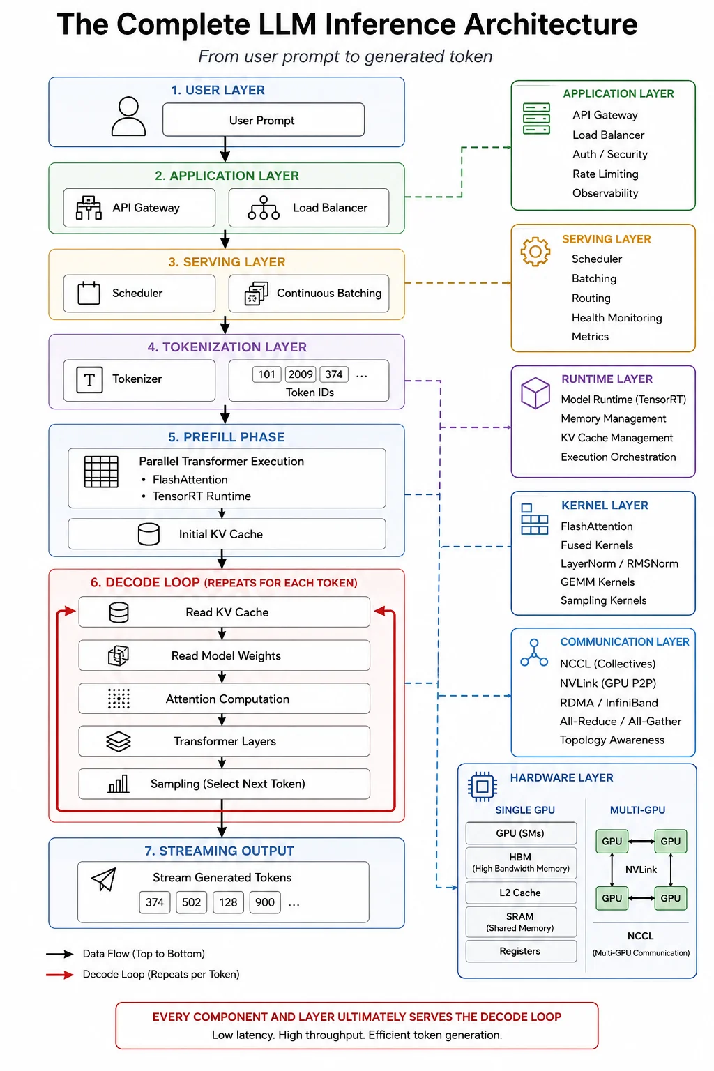
The Lifecycle of a Request
The Infrastructure Layers
Each step in the lifecycle executes inside one of six distinct infrastructure layers:
2. Why Inference Is Harder Than It Looks
A common misconception is that serving an AI model is simply running the training loop forward. In reality, the two workloads stress the hardware in completely opposite ways.
- Compute-bound: data flows in massive, predictable, static batches
- GPUs spend almost all time performing matrix math
- Tensor Cores stay saturated
- Batch sizes are large and fixed
- Context lengths are known upfront
- Memory-bound: requests arrive randomly with unpredictable lengths
- GPUs spend most time waiting for data from memory
- Tensor Cores sit idle between memory fetches
- Batch sizes are small and variable
- Generation length is unknown until the model finishes
Because of these realities, companies increasingly invest more engineering effort in serving infrastructure than in model training infrastructure. The physics of serving dictate the economics of the entire product, and a model that generates at 5 tokens per second is unusable in a chat product regardless of its quality.
3. Prompt Arrival: Load Balancing and Continuous Batching
The lifecycle of an LLM response begins long before the GPU spins up. When you hit Enter, your text is encapsulated in an API request routed to an inference cluster.
Network and Routing
In a production environment, your request first hits a load balancer. LLMs are largely stateless across requests, so the load balancer routes your prompt to the inference server with the most available capacity. For latency-sensitive applications, this routing also considers geographic proximity: a request from Tokyo should not traverse to a US datacenter when a regional node is available.
The Scheduler and Continuous Batching
Once the inference server receives the request, it enters a queue. In traditional deep learning, batching is static: you wait for 8 requests to arrive, pad them to the same length, and run them together. For LLMs, this is highly inefficient because sequences have unpredictable generation lengths. One request might generate "Yes," while another generates a 500-word essay.
To maximize throughput, modern inference servers use continuous batching (also called iteration-level scheduling). Instead of waiting for an entire batch to finish, the scheduler operates at the token level. The moment a sequence emits an end-of-sequence token, it is immediately evicted from the batch and a new request is slotted in its place. This drastically improves GPU utilization and handles concurrent users efficiently.
4. Tokenization: From Text to Integer IDs
GPUs do not understand text: they understand numbers. Before your prompt can touch the model, it must be converted into a sequence of integers through tokenization.
Text to Tokens
Modern LLMs use subword tokenization algorithms like Byte Pair Encoding (BPE) or SentencePiece. These algorithms learn statistical representations of text, compressing common words into single tokens while breaking rare words into subword pieces.
Consider the word "unbelievable". A tokenizer might split it into three tokens: un, believ, able. Each is mapped to a specific integer ID in the model's vocabulary, for example [345, 8712, 1102]. The full vocabulary of modern models typically contains 32,000 to 128,000 unique tokens.
Why Token Count Drives Cost, Latency, and Limits
In LLM systems, token count is the fundamental unit of everything:
- Cost: API providers charge per token because every token requires a fixed amount of compute and memory access.
- Latency: More tokens in your prompt means a longer prefill phase and higher Time To First Token.
- Context window: Models have a hard mathematical limit on how many tokens they can process at once: the context window (e.g., 8k, 32k, 128k tokens).
5. Prefill vs Decode: The Two Phases of Generation
Once tokenized, the sequence enters the neural network. LLM inference is split into two fundamentally different execution phases with opposing hardware profiles.
The Prefill Phase
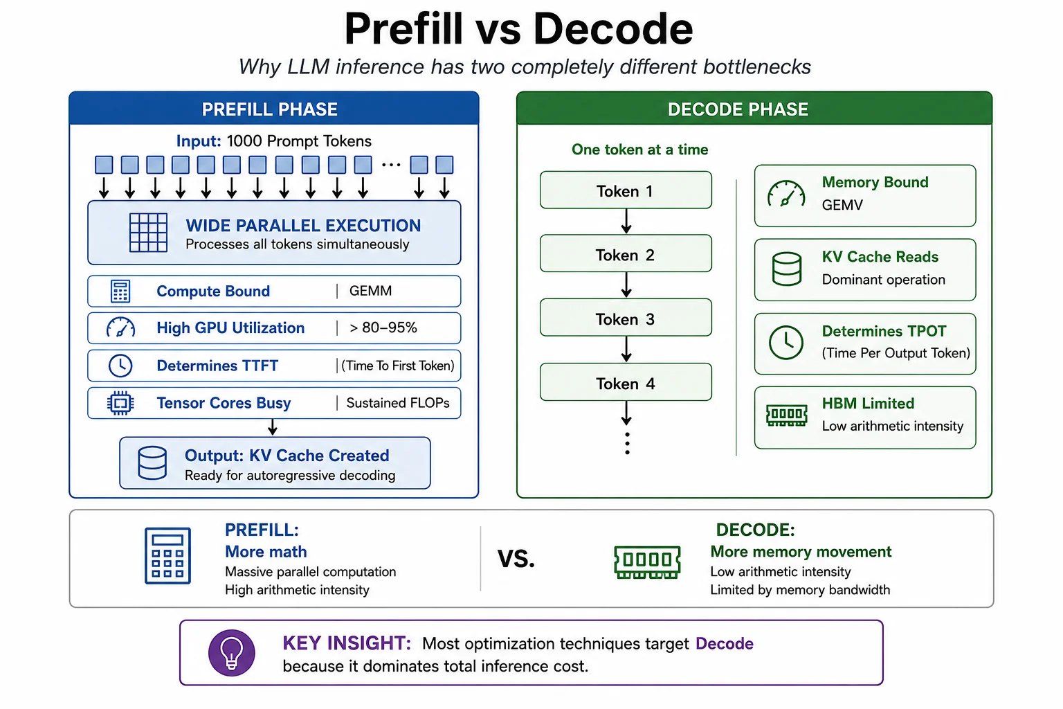
Prefill is the ingestion of your entire prompt. Because all input tokens are known upfront, the GPU processes them in parallel. During this forward pass, the model does two things simultaneously: calculates the probability distribution for the very first token to generate, and builds the attention state (the KV cache) for every input token. The prefill phase is compute-bound and dictates your Time To First Token (TTFT).
The Decode Phase
Decode is fundamentally different. The model can only generate one token at a time: it cannot predict token 3 without first knowing token 2. For every single generated token, the GPU must load the entire model weight set and the entire KV cache from memory, perform a relatively small matrix-vector multiplication, and write back one new token. The decode phase is memory-bound and dictates your tokens-per-second output rate (TPOT).
| Characteristic | Prefill (Processing the Prompt) | Decode (Generating the Response) |
|---|---|---|
| Parallelism | High: all prompt tokens simultaneously | Low: one token at a time, sequentially |
| Compute Pattern | Matrix-Matrix Multiplication (GEMM) | Matrix-Vector Multiplication (GEMV) |
| Bottleneck | Compute-bound (GPU FLOPS) | Memory-bound (HBM bandwidth) |
| GPU Utilization | High: Tensor Cores saturated | Low: Tensor Cores wait for memory |
| Latency Metric | Time To First Token (TTFT) | Time Per Output Token (TPOT) |
| KV Cache Usage | Writes heavily to cache | Reads heavily; writes 1 new entry per token |
| Scaling Behavior | Cost grows quadratically with prompt length | Cost grows linearly with generation length |
Understanding this split is arguably the most important concept in AI infrastructure. The same GPU must excel at two completely different workloads within a single request, and optimizing one often comes at the cost of the other.
6. Transformer Attention Deep Dive: Q, K, V
To understand why the KV Cache exists, you must first understand the math of transformer attention during inference.
Query, Key, and Value
In a transformer, attention allows every token to gather context from all other tokens in the sequence. Every token produces three vectors:
- Query (Q): What information am I looking for?
- Key (K): What information do I contain?
- Value (V): What is my underlying content/meaning?
Attention scores are computed as:
During generation, when predicting token N+1, the model generates a single Query for the current token. To understand context, this Query must attend to the Keys and Values of all preceding tokens (0 through N).
Why This Forces Caching
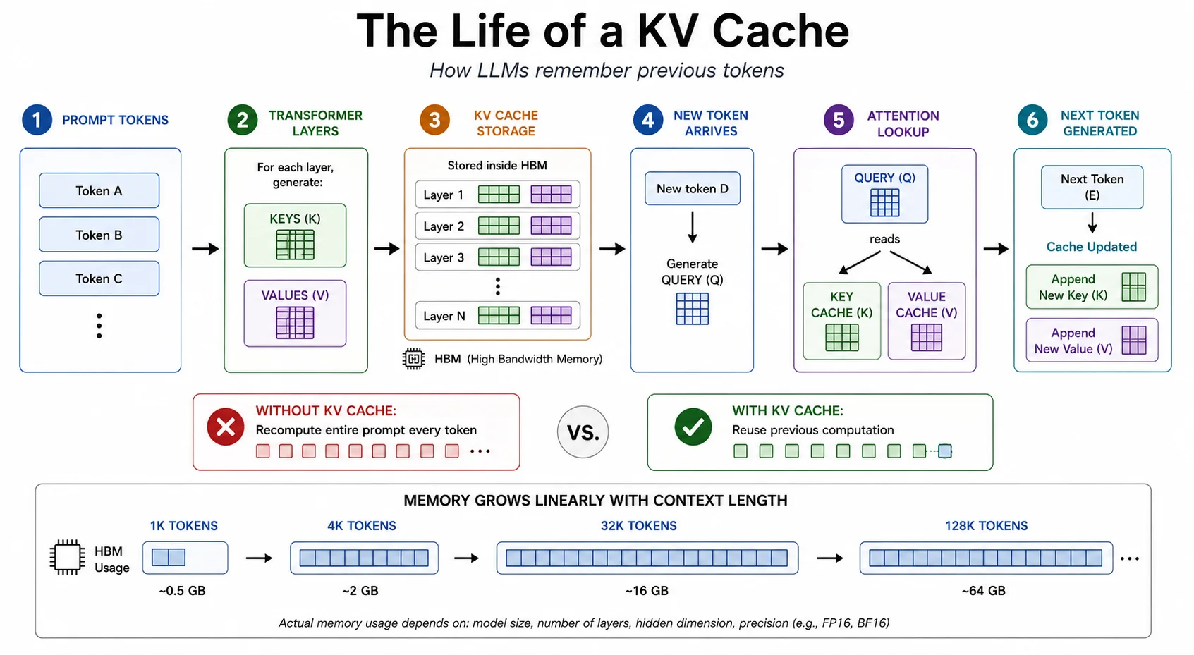
If Keys and Values were not saved, the model would have to rerun the entire sequence through the neural network for every new word, resulting in O(N²) computational complexity for generation. By caching K and V tensors, generating the next token becomes O(N). This is the KV cache. Without it, even a 100-token response would require running 5,050 forward passes instead of 100.
7. The KV Cache: Why It Exists and What It Costs
The KV cache prevents exponential compute costs, but it introduces massive GPU memory requirements. Understanding this trade-off is central to every inference infrastructure decision.
What Determines KV Cache Size
Cache size is determined entirely by architecture parameters; it is independent of model weight size:
- Number of layers: deeper models cache states at every layer
- Number of KV heads: determines how many attention vectors are stored
- Head dimension: the size of each K and V vector
- Precision format: FP16 (2 bytes), FP8 (1 byte)
- Context length: total tokens processed and generated
The Math: Why GPT-3 Scale Was Unsustainable
For a traditional Multi-Head Attention model like GPT-3 (96 layers, 96 heads, 128 head-dim, FP16):
For a single user with an 8,000-token context:
An NVIDIA A100 has 80 GB of total VRAM. Without architectural optimization, a single GPU could barely serve two concurrent users. This made large-context serving economically impossible.
The Modern Reality: Llama 3 with GQA
Modern models solve this by drastically reducing KV heads. Llama 3 70B uses 80 layers, head-dim 128, FP16, but only 8 KV heads instead of 64:
By changing the attention architecture, the per-user memory footprint dropped from 37.7 GB to 2.6 GB, a 14× reduction that makes dozens of concurrent users viable on the same hardware.
8. Grouped Query Attention: MHA to GQA
The dramatic memory reduction shown above comes from Grouped Query Attention (GQA), the architectural change that made large-context inference financially viable.
During decode, the GPU must stream the entire KV cache from HBM to compute cores for every token generated. A smaller cache means less data to move, directly translating to faster generation speeds. GQA is why modern frontier models can run long-context inference at commercially viable speeds.
9. PagedAttention and Prefix Caching
PagedAttention: Eliminating Memory Waste
Even with GQA, dynamically allocating KV cache memory is complex. Early inference systems allocated memory for the maximum possible sequence length contiguously upfront. If a slot was reserved for 2,048 tokens but the model generated only 10, the remaining 2,038 slots were wasted, causing internal fragmentation that was destroying GPU utilization.
PagedAttention borrows the concept of virtual memory from operating systems. The cache is divided into small, fixed-size blocks (typically 16 tokens per block). The GPU allocates these blocks non-contiguously on demand, linking them via a block table. This practically eliminates memory waste and allows vLLM to serve far more concurrent requests on the same hardware.
Prefix Caching: Reusing Work Across Requests
Many production workloads send requests that share identical starting tokens. A customer service bot with a large system prompt, or a RAG pipeline inserting the same document into multiple concurrent queries, will rebuild identical KV cache states for those shared tokens on every single request, wasting compute and memory bandwidth.
Prefix caching allows the serving engine to recognize identical token sequences and reuse previously computed KV states. By storing shared prefixes in HBM, engines like vLLM and SGLang skip the most expensive part of the prefill phase entirely.
The practical results are significant: reduced TTFT, lower compute costs per request, and massively improved multi-user throughput, especially for RAG and agent pipelines that reuse the same context repeatedly.
10. The GPU Memory Stack
Before isolating the ultimate hardware bottleneck, you need a clear picture of where data actually lives inside a GPU. The GPU memory hierarchy dictates almost all modern inference optimizations.
Moving data is significantly slower and more power-hungry than performing math on it. As data moves further from the compute cores, latency skyrockets and bandwidth plummets:
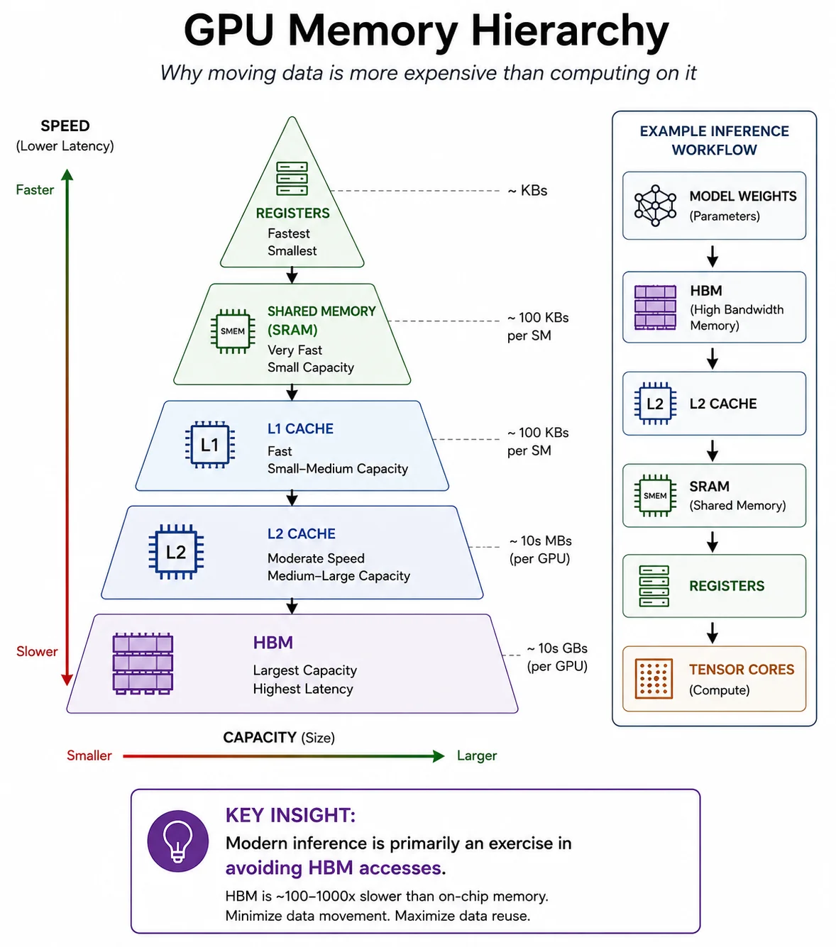
Optimizing inference is fundamentally a battle to keep model weights and KV cache data in Registers and SRAM for as long as possible, avoiding the latency penalty of constantly reading from and writing to HBM. Every major inference kernel optimization is a variation on this theme.
11. HBM: The Real Bottleneck of LLM Inference
When discussing GPU performance, mainstream coverage focuses on FLOPS. In LLM generation, FLOPS hardly matter. The actual bottleneck is High Bandwidth Memory (HBM).
GPU Bandwidth Comparison
| GPU | HBM Capacity | Memory Bandwidth | Relative Throughput |
|---|---|---|---|
| NVIDIA A100 | 80 GB | 2.0 TB/s | 1.0× |
| NVIDIA H100 | 80 GB | 3.35 TB/s | ~1.7× |
| NVIDIA H200 | 141 GB | 4.8 TB/s | ~2.4× |
| NVIDIA B200 | 192 GB | 8.0 TB/s | ~4× |
Relative throughput normalized to A100 baseline. Real throughput depends on batch size, quantization, and KV cache size.
For large language models, inference is often memory-bandwidth bound rather than compute-bound. During token generation, the GPU must repeatedly stream model weights from HBM into compute units. If the active model weights and KV cache together occupy roughly 100 GB, an H100 with 3.35 TB/s of memory bandwidth can move that data in about 30 ms, implying an upper bound of roughly 33 tokens per second for a single sequential request. In practice, optimizations, batching, quantization, and cache reuse can improve throughput, but memory bandwidth remains a primary bottleneck for large models. This is why GPUs such as the H200, which significantly increase memory capacity and bandwidth while offering only modest compute improvements, can deliver substantial real-world inference speedups for large-scale LLM workloads.
GPU Occupancy and Warp Scheduling
A GPU is divided into Streaming Multiprocessors (SMs). Each SM manages execution in groups of 32 threads called warps. To hide memory latency, an SM needs multiple warps loaded simultaneously: while one warp waits for data to arrive from HBM, the SM swaps to another warp. If there are not enough active warps, the SM stalls and compute throughput collapses.
Inference workloads frequently suffer from low occupancy when serving a single user. By grouping 64 or 128 requests into a batch via continuous batching, the matrix sizes grow large enough to fill all SMs, amortizing the cost of reading model weights across many users simultaneously.
12. Triton and FlashAttention: Kernel-Level Optimization
The Triton Language
Standard framework code runs inefficiently on GPUs. To extract maximum performance, engineers write specialized software routines called kernels. Historically this meant writing CUDA, notoriously complex and error-prone. The Triton language, developed by OpenAI, allows engineers to write fast GPU kernels in Python while retaining direct control over SRAM and HBM access patterns.
Kernel Fusion
In standard PyTorch, operations execute sequentially. An addition followed by layer normalization writes the addition result back to HBM, then reads it back into SRAM for normalization, a round trip that destroys latency. Kernel fusion eliminates this: a fused Triton kernel loads data into SRAM once, performs the addition, runs the normalization, applies the activation, and only then writes the final result back to HBM. One trip instead of four.
FlashAttention: Tiling the Attention Matrix
Standard attention computes an N×N matrix where N is sequence length. For a 10,000-token context, that is a 100-million element matrix written to HBM and read back, catastrophically slow. FlashAttention solves this using tiling.
Instead of computing the whole matrix at once, the FlashAttention kernel breaks Queries, Keys, and Values into small tiles that fit entirely inside the GPU's SRAM. It computes attention for each tile, updates a running sum, and moves to the next, without ever materializing the full N×N matrix in HBM. Memory reads and writes drop from O(N²) to O(N), dramatically accelerating the prefill phase and enabling practical long-context inference.
13. TensorRT and Quantization
TensorRT: Compiling for the Hardware
Before a model is deployed to production, it undergoes a compilation phase. TensorRT takes the model's neural network graph and acts as an optimizing compiler. It analyzes the specific GPU it will run on, tests hundreds of different low-level kernel algorithms, and selects the fastest implementation for each layer of the specific model architecture. The result is a compiled engine that runs significantly faster than the original framework code.
Quantization: Halving the Memory Problem
Since generation is memory-bound, reducing the size of what gets moved from HBM is a direct performance multiplier. Quantization converts model weights from 16-bit floats (FP16) to 8-bit integers (INT8) or 8-bit floats (FP8).
The arithmetic is straightforward: FP16 to FP8 halves the bytes per parameter. A 70B model in FP16 consumes ~140 GB. Quantized to FP8, it consumes ~70 GB, fitting on a single H100 that previously required two GPUs. Every token now requires moving half as many bytes from HBM, theoretically doubling generation speed while fitting twice as many concurrent users on the same cluster.
14. Speculative Decoding: Generating Multiple Tokens per Step
The fundamental bottleneck of autoregressive generation (where each token is predicted from all previous tokens, one at a time) is sequentiality: one token at a time. The entire memory-bound decode cycle must run end-to-end for every single word. Speculative decoding breaks this constraint by generating multiple tokens per step without degrading output quality.
How It Works
Speculative decoding pairs a small, fast "draft" model with the large "target" model:
- The draft model rapidly predicts a sequence of future tokens (e.g., 4 tokens ahead). Because it is small, this is cheap and fast.
- The target model takes this proposed sequence and runs a single parallel forward pass to verify all tokens at once.
- Accepted tokens are immediately emitted. If the draft guessed incorrectly at token 3, the target rejects from that point forward and inserts the correct token.
Because validating a batch of tokens in parallel is far cheaper than generating them one-by-one, speculative decoding can double or triple tokens-per-second throughput. It is now a standard technique in frontier production systems, used by Google, Anthropic, and Meta for their inference pipelines.
15. Where Inference Time Actually Goes: TTFT vs TPOT
When a user complains about slow generation, where is the time actually being spent? System architects break inference latency into two distinct metrics that must be optimized entirely differently.
- How long until the first word appears
- Dominated by prefill compute and queueing delay
- Critical for interactive chat applications
- Optimized via FlashAttention, chunked prefill, prefix caching
- Interval between each subsequent token
- Dominated by HBM bandwidth during decode
- Critical for bulk / throughput workloads
- Optimized via quantization, GQA, speculative decoding
| Stage | Metric | Primary Bottleneck | Key Optimizations |
|---|---|---|---|
| Network | TTFT | Physical distance / ISP | Edge routing, regional datacenters |
| Tokenization | TTFT | CPU parsing speed | Fast tokenizers written in Rust or C++ |
| Queueing | TTFT | Concurrent load | Continuous batching, admission control |
| Prefill | TTFT | GPU FLOPS (compute-bound) | FlashAttention, chunked prefill |
| KV Cache Reads | TPOT | HBM capacity and bandwidth | PagedAttention, GQA, KV quantization |
| Decode | TPOT | HBM bandwidth (memory-bound) | Weight quantization (FP8/INT8) |
| Sampling | TPOT | CPU/GPU sync overhead | Fused logits kernels |
| Multi-GPU Sync | TPOT | Interconnect latency | NVLink, NCCL AllReduce tuning |
| Streaming | TPOT | Network connection | Server-Sent Events (SSE) optimization |
Interactive applications (chatbots, copilots) prioritize low TTFT: users are sensitive to initial delays and will abandon sessions that feel unresponsive. Enterprise workloads (batch summarization, document processing) care about overall throughput: low TPOT means higher requests per second, lower GPU cost per output token.
16. The Four Bottlenecks Framework
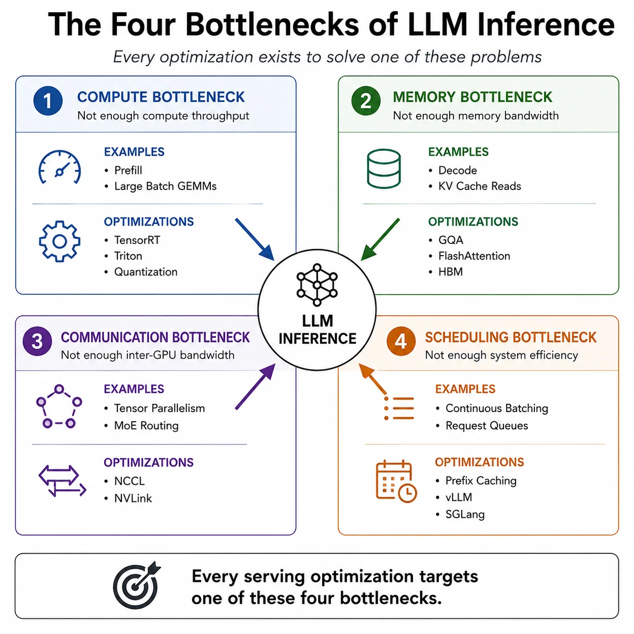
Almost every inference performance problem reduces to one of four fundamental system bottlenecks. Having a clear mental framework for these is essential for diagnosing production issues and knowing which optimization to reach for first.
Conclusion: Engineering the Response
Every word an LLM streams to you is the result of a precisely coordinated systems pipeline fighting against the fundamental physics of data movement. The model is not the hard part: the infrastructure around it is.
- Prefill is compute-bound: all tokens in parallel, building the attention state that makes generation possible.
- Decode is memory-bound: one token at a time, reading gigabytes of weights and cache from HBM for every single word.
- The KV cache prevents O(N²) compute at the cost of O(N) memory, the central trade-off of modern LLM serving.
- GQA, PagedAttention, FlashAttention, quantization, and speculative decoding all attack the same constraint: how many bytes the GPU has to move per token.
The engineers shipping the fastest AI products are not the ones with the largest models: they are the ones who most deeply understand the memory hierarchy, the batching scheduler, and the kernel optimizations that determine how many tokens per second their hardware can produce. That understanding is what this article builds toward.
Frequently Asked Questions
What is the difference between prefill and decode?
Prefill processes your entire input prompt in parallel and is compute-bound: it determines Time To First Token (TTFT). Decode generates one token at a time by reading model weights and the KV cache from memory on every step, and is memory-bound: it determines how fast tokens stream back to you (TPOT). The same GPU executes both phases within a single request.
Why is LLM inference memory-bound rather than compute-bound?
During decode, generating each token requires loading the model's full weight set and KV cache from HBM to compute cores. The math itself is a single matrix-vector multiply. The bottleneck is how fast the GPU can shuttle bytes, not how fast it can do arithmetic. An H100 can theoretically perform 1,979 TFLOPS of BF16 compute but can only move 3.35 TB/s of data. For large models, the data movement is the ceiling.
What happens when the KV cache fills up?
When the KV cache exhausts GPU VRAM, the serving engine must evict sequences. Less sophisticated systems will reject new requests or return out-of-memory errors. More advanced systems (like vLLM with PagedAttention) can swap low-priority blocks to CPU RAM, though this comes with significant latency penalties. This is why KV cache memory management (through GQA, quantization, and PagedAttention) is central to production LLM infrastructure.
Does speculative decoding change the model output?
Speculative decoding is provably mathematically equivalent to standard autoregressive sampling. The target model verifies every draft token, and rejected tokens are replaced with the target model's correct prediction. The output distribution is identical to running the large model alone. The only change is speed: fewer sequential decode steps for the same number of generated tokens.
What is vLLM and why does it matter?
vLLM is an open-source LLM serving engine developed at UC Berkeley that popularized PagedAttention and continuous batching. It is the most widely deployed open-source inference server, running models from Llama to Mistral to Qwen in production across thousands of organizations. Understanding vLLM's architecture gives you a concrete implementation of almost every concept covered in this article: continuous batching, PagedAttention, prefix caching, and speculative decoding.