Quantum Machine Learning
QML uses parameterized quantum circuits trained by classical optimizers, with variational classifiers as the main model
Source: mortalapps.com- Quantum Machine Learning merges quantum mechanics with classical optimization to build parameterized quantum models.
- Variational Quantum Classifiers (VQCs) use classical optimizers to update quantum gate parameters based on measurement feedback.
- The parameter-shift rule allows exact gradients to be calculated directly on quantum hardware without numerical approximation.
- Ewin Tang's dequantization results proved that many claimed quantum speedups in ML can be matched by quantum-inspired classical algorithms.
- The 'input bottleneck' of encoding large classical datasets into quantum states remains a major practical hurdle.
- Barren plateaus represent a critical challenge where gradients vanish exponentially as the number of qubits scales.
Why This Matters
Welcome to the frontier of quantum computing. Over the past nine sections, you have journeyed from the foundational mathematics of Hilbert spaces to the complex engineering of fault-tolerant quantum error correction. Now, we stand at the boundary of current human knowledge to explore how these systems will reshape our technological landscape. We begin this final section with Quantum Machine Learning (QML), an area of intense research that seeks to merge the computational power of quantum mechanics with the predictive capabilities of artificial intelligence.
Core Intuition
To understand Quantum Machine Learning, imagine trying to find a pattern in a highly complex, multi-dimensional dataset. In classical machine learning, we often project data into higher dimensions using kernel methods to make it linearly separable, like trying to find a flat line that separates two interlocked shapes by looking at their shadows on a wall. A quantum computer acts as an exponentially large linear algebra engine, allowing us to map classical data into a Hilbert space of $2^N$ dimensions using only $N$ qubits. This massive state space provides a natural environment for identifying complex correlations that are classically invisible.
Another helpful analogy is to think of a parameterized quantum circuit as a highly adjustable physical instrument, like a complex synthesizer. By turning the knobs (the gate parameters), we change the interference patterns of the quantum states. Our goal is to tune these knobs so that the constructive interference aligns with the correct classifications of our data, while destructive interference suppresses incorrect predictions. This process of tuning quantum parameters using classical feedback loops is the core mechanism of variational quantum algorithms.
Visualization
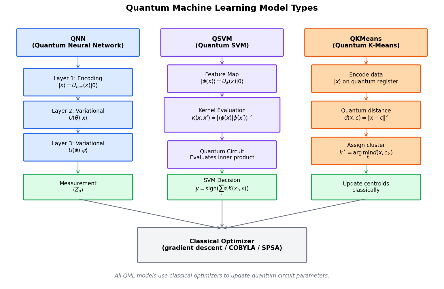
Technical Explanation
At the heart of near-term QML is the Variational Quantum Classifier (VQC). The process begins with classical data $x$, which must be encoded into a quantum state $| \psi(x) \rangle$ using a feature map $U_{\Phi}(x)$. A common choice is amplitude encoding, which maps an $M$-dimensional classical vector to the amplitudes of an $N$-qubit state where $N = \lceil \log_2 M \rceil$. Once the state is prepared, we apply a parameterized ansatz $V(\theta)$, consisting of single-qubit rotations and entangling gates. The final state is given by:
$$| \psi(x, \theta) \rangle = V(\theta) U_{\Phi}(x) | 0 \rangle^{\otimes N}$$
We then measure the expectation value of an observable $M$, yielding the model's prediction:
$$f(x, \theta) = \langle \psi(x, \theta) | M | \psi(x, \theta) \rangle$$
To train the model, we define a classical loss function $L(\theta)$ and compute its gradients with respect to the parameters $\theta$. Because we cannot directly backpropagate through a physical quantum circuit, we use the parameter-shift rule to calculate exact gradients on the hardware:
$$\frac{\partial f(x, \theta)}{\partial \theta_i} = \frac{f(x, \theta_i + \frac{\pi}{2}) - f(x, \theta_i - \frac{\pi}{2})}{2}$$
While QML offers theoretical exponential speedups for specific tasks, the field was profoundly challenged by Ewin Tang's 2018 'dequantization' results. Tang demonstrated that many quantum machine learning algorithms (such as recommendation systems) could be replicated classically in polynomial time using classical algorithms inspired by quantum sampling techniques. This highlighted the critical need for rigorous benchmarks and proved that quantum advantage in ML is not guaranteed simply by using quantum states.