Multiple Measurements
A single measurement yields one classical bit, so reconstructing a quantum state requires many identical preparations
Source: mortalapps.com- A single quantum measurement yields only a single classical bit, destroying the superposition.
- To reconstruct a quantum state, we must measure an ensemble of identically prepared qubits.
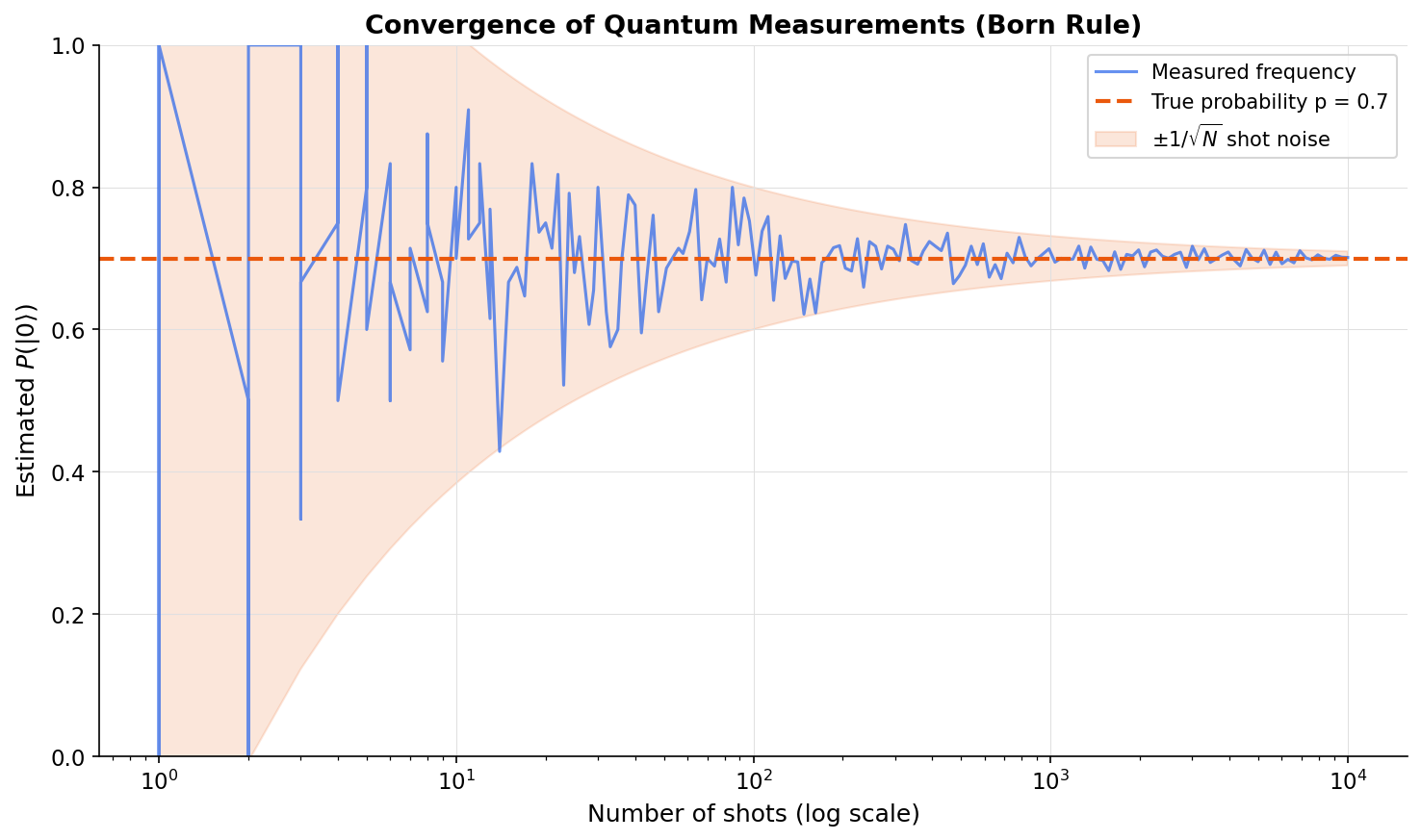
- The experimental frequency of outcomes converges to the Born Rule probabilities as the number of shots increases.
- The statistical error of quantum measurement scales as 1/√N, where N is the number of shots.
- The expectation value ⟨A⟩ is the average outcome of measuring an observable A over many trials.
- Quantum state tomography is the process of fully reconstructing a state vector by measuring in multiple bases.
Why This Matters
Because quantum mechanics is fundamentally probabilistic, a single measurement of a qubit in superposition yields very little information. It simply gives you a 0 or a 1, completely destroying the superposition in the process. To understand the true state of a qubit before collapse, we must adopt a statistical approach. We must prepare the exact same state over and over again, measuring it each time to build up a detailed probability distribution.
In this topic, we will explore the mathematics of multiple measurements. We will study how the Law of Large Numbers applies to quantum systems, allowing us to reconstruct the amplitudes $\alpha$ and $\beta$ from experimental data. We will define the concept of expectation values and understand how repeated trials allow us to verify quantum algorithms with high statistical confidence.
By the end of this topic, you will be able to calculate the expectation value of a quantum operator, determine the statistical error of a set of measurements, and explain the process of quantum state tomography, the method used to read out the complete state of a quantum processor.
Core Intuition
Imagine you are handed a biased coin, and you want to find out exactly how biased it is. If you flip it once and get heads, you have learned almost nothing. The coin could be 51% heads, 99% heads, or even a fair 50/50 coin. But if you flip the coin 1,000 times and get heads 750 times, you can state with high confidence that the coin has a 75% bias toward heads. This is the core intuition of multiple measurements.
In quantum computing, we cannot 're-flip' the same qubit because the first measurement collapsed it. Instead, we use a factory-like approach. We use our quantum computer to prepare a qubit in a specific state, measure it, and record the result. Then, we reset the system, prepare the *exact same* state again, and measure it. We repeat this process thousands of times.
Each individual run is called a 'shot.' By counting the ratio of 0s to 1s across all shots, we can reconstruct the squared magnitudes of our amplitudes. If we want to find the phase, we repeat this entire process but rotate the qubits before measuring them. This statistical reconstruction is how we read the output of a quantum computer.
Visualization
Technical Explanation
Let us formalize this statistically. Suppose we prepare a qubit in the state $|\psi\rangle = \alpha|0\rangle + \beta|1\rangle$ and measure it in the computational basis $N$ times. Each measurement is an independent Bernoulli trial.
Let $N_0$ be the number of times we measure 0, and $N_1$ be the number of times we measure 1, such that $N_0 + N_1 = N$. According to the Law of Large Numbers, as the number of measurements $N$ approaches infinity, the experimental frequencies converge to the theoretical probabilities:
$$\lim_{N \to \infty} \frac{N_0}{N} = P(0) = |\alpha|^2$$ $$\lim_{N \to \infty} \frac{N_1}{N} = P(1) = |\beta|^2$$
For a finite number of measurements $N$, the statistical error (standard deviation) scales as $1/\sqrt{N}$. This means to double our precision, we must quadruple the number of shots.
We also define the expectation value of an observable (represented by a Hermitian matrix $A$). The expectation value, denoted as $\langle A \rangle$, is the average outcome we expect to measure over many trials:
$$\langle A \rangle = \langle\psi|A|\psi\rangle$$
For example, if we measure the Pauli-Z operator $Z = \begin{pmatrix} 1 & 0 \\ 0 & -1 \end{pmatrix}$ (which has eigenvalues +1 for $|0\rangle$ and -1 for $|1\rangle$):
$$\langle Z \rangle = \langle\psi|Z|\psi\rangle = |\alpha|^2(1) + |\beta|^2(-1) = |\alpha|^2 - |\beta|^2$$
This value ranges from +1 (definitely 0) to -1 (definitely 1), with 0 representing a perfect 50/50 superposition.