Quantum Fourier Transform

The Quantum Fourier Transform (QFT) is the quantum analogue of the classical Discrete Fourier Transform (DFT). It is not an algorithm designed to solve a standalone problem, but rather a powerful subroutine that underpins many of the most famous quantum algorithms, including Shor's factoring algorithm and Quantum Phase Estimation.

Imagine a clock with a single hand. If you set the clock to 3 o'clock, that is a discrete, localized state. The classical Fourier transform takes a sequence of such positions and finds the underlying frequencies. The Quantum Fourier Transform does this directly on the state of qubits. Instead of representing a number $j$ as a binary string (like $|011\rangle$), the QFT encodes $j$ as a series of phase rotations on the qubits. Qubit 1 rotates by a half-turn, Qubit 2 by a quarter-turn, and Qubit 3 by an eighth-turn. By translating localized computational states into distributed phase patterns, the QFT allows us to detect periodic patterns in quantum states with exponential efficiency.

The Discrete Fourier Transform (DFT) maps a vector of complex numbers $(x_0, \dots, x_{N-1})$ to $(y_0, \dots, y_{N-1})$ according to:

$$y_k = \frac{1}{\sqrt{N}} \sum_{j=0}^{N-1} x_j e^{2\pi i j k / N}$$

The Quantum Fourier Transform (QFT) performs this exact transformation on the amplitudes of a quantum state. It maps the basis state $|j\rangle$ to a superposition of basis states:

$$|j\rangle \mapsto \text{QFT}|j\rangle = \frac{1}{\sqrt{N}} \sum_{k=0}^{N-1} e^{2\pi i j k / N} |k\rangle$$

where $N = 2^n$.

Product Representation: To implement this as a circuit, we can rewrite the QFT state in a product form:

$$|j\rangle \mapsto \frac{1}{\sqrt{2^n}} \left( |0\rangle + e^{2\pi i 0.j_n} |1\rangle \right) \otimes \dots \otimes \left( |0\rangle + e^{2\pi i 0.j_1 j_2 \dots j_n} |1\rangle \right)$$

where $0.j_1 j_2 \dots j_n = \sum_{l=1}^n j_l 2^{-l}$ is binary fraction notation.

Complexity Comparison:

• Classical FFT: $O(N \log N) = O(n 2^n)$ operations.
• Quantum QFT: $O(n^2)$ gates.

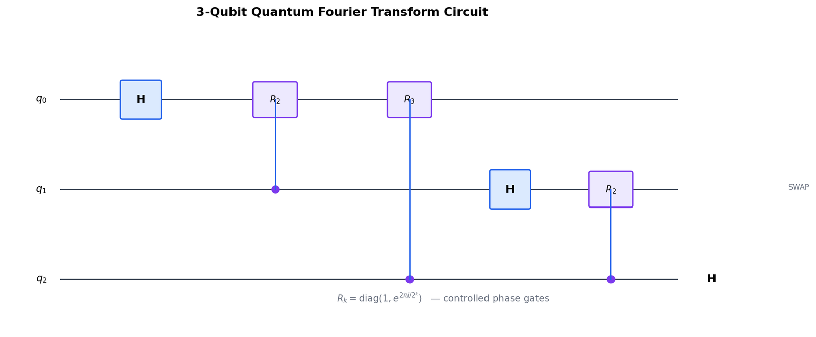
Circuit Construction: The QFT circuit is constructed using Hadamard gates ($H$) and controlled phase rotation gates ($R_k$), where:

$$R_k = \begin{pmatrix} 1 & 0 \\ 0 & e^{2\pi i / 2^k} \end{pmatrix}$$

For each qubit $i$ (from $1$ to $n$): 1. Apply $H$ to qubit $i$. 2. For each remaining qubit $j > i$, apply a controlled-$R_{j-i+1}$ gate with qubit $j$ as control and qubit $i$ as target. 3. Reverse the order of the qubits at the end using SWAP gates.