Measuring Results
Measurement results are probabilistic bitstrings in count dictionaries, requiring statistical analysis across many shots
Source: mortalapps.com- Quantum measurement collapses superpositions into classical bitstrings, making results fundamentally probabilistic.
- Qiskit aggregates measurement outcomes into counts dictionaries, mapping binary strings to their observed frequencies.
- The experimental probability of an outcome is calculated as its count divided by the total number of shots.
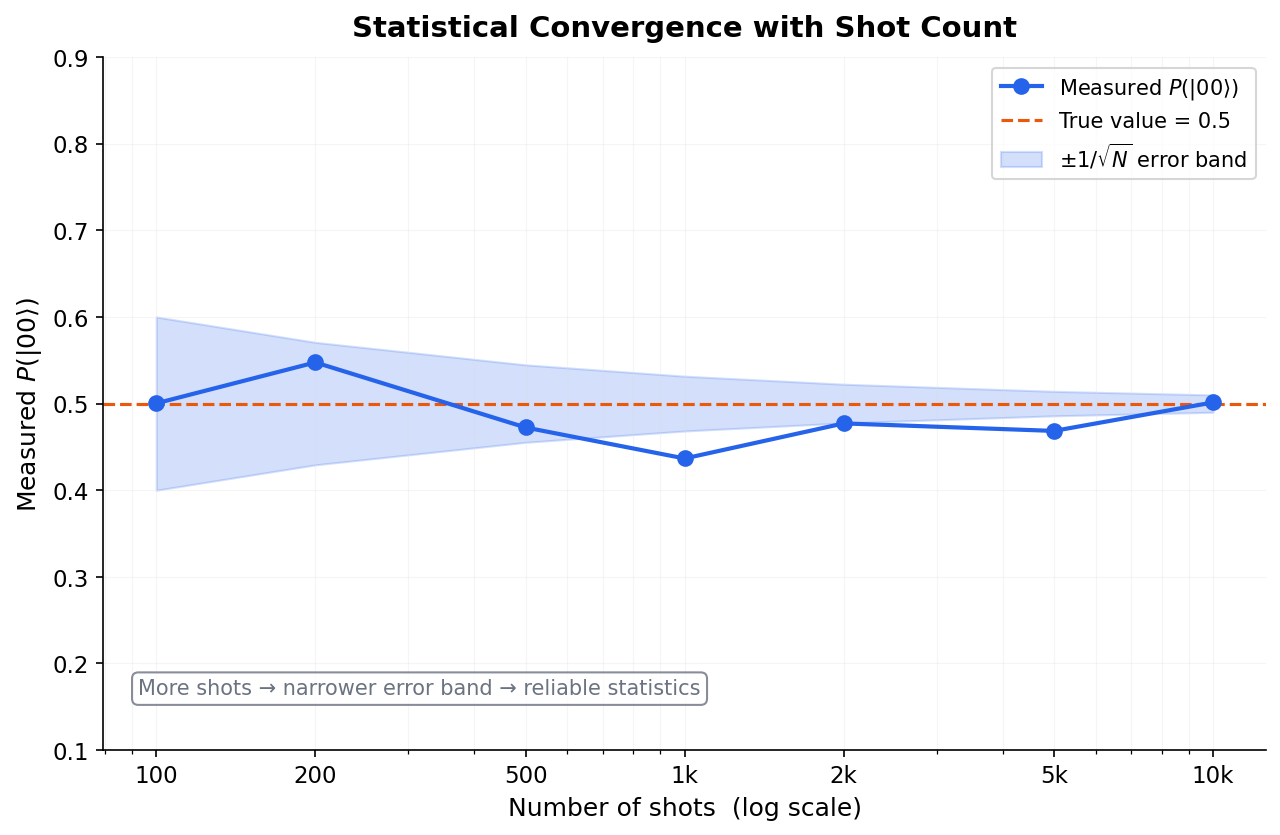
- Statistical sampling error (shot noise) scales as $1/\sqrt{N}$, meaning precision increases with the square root of the shot count.
- To halve the statistical margin of error, you must increase the number of shots by a factor of four.
- Qiskit Primitives return quasi-probabilities, which apply error mitigation to correct for physical hardware readout errors.
Why This Matters
The ultimate goal of any quantum program is to extract classical information that solves a computational problem. Because quantum states exist in superposition, we cannot access their probability amplitudes directly. Instead, we must perform physical measurements, which collapse the quantum state into classical bits. This process is fundamentally probabilistic, meaning that analyzing quantum results requires statistical methods.
When a quantum circuit is executed for multiple shots, the output is a collection of classical bitstrings. Qiskit aggregates these outcomes into structured data formats, primarily 'counts' dictionaries and 'quasi-probability' distributions. Interpreting this data correctly requires understanding the physics of measurement collapse, the mathematics of probability distributions, and the statistical noise inherent in finite sampling.
In this topic, you will learn how to extract and analyze measurement data in Qiskit 1.x. You will understand how to read counts dictionaries, calculate experimental probabilities, and analyze statistical error (shot noise). You will write code to process results from multi-qubit measurements and learn how to distinguish true quantum correlations from random statistical fluctuations.
Core Intuition
Think of measuring a quantum circuit like conducting a political opinion poll. You cannot read the minds of the entire population (the quantum statevector) simultaneously. Instead, you call a random sample of 1000 voters (the shots) and ask them a yes/no question (the measurement). Each phone call collapses that voter's state into a single classical answer: 'Yes' (1) or 'No' (0).
If your poll returns 510 'Yes' and 490 'No' answers, you don't assume the population is exactly split 51% to 49%. You know there is a margin of error (statistical noise) due to your finite sample size. If you want a more precise estimate, you must call more voters (increase the shot count). The margin of error shrinks as you gather more data, following the law of large numbers.
In Qiskit, the counts dictionary is your poll tally sheet (e.g., {'00': 512, '11': 512}). The quasi-probability distribution is your calculated percentage (e.g., {'00': 0.5, '11': 0.5}), adjusted for any known biases in your polling method. By analyzing these distributions, you can reconstruct the underlying quantum state with high statistical confidence.
Visualization
Technical Explanation
According to the Born Rule, the probability of measuring a quantum state $\lvert \psi \rangle$ and obtaining the classical outcome $i$ is given by:
$$P(i) = \lvert \langle i \lvert \psi \rangle \rvert^2$$
When we run a circuit for $N$ shots, we obtain an experimental count $C_i$ for each outcome $i$. The experimental probability (or frequency) is:
$$\hat{P}(i) = \frac{C_i}{N}$$
Due to statistical sampling noise (shot noise), the experimental probability $\hat{P}(i)$ fluctuates around the true theoretical probability $P(i)$. The statistical standard deviation (standard error) of this estimate scales as:
$$\sigma \approx \frac{1}{\sqrt{N}}$$
To halve your statistical error, you must quadruple your shot count. In Qiskit 1.x, the Sampler primitive returns quasi-probabilities, which are probabilities that have been mathematically processed to mitigate hardware readout errors, meaning they can occasionally have small negative values in highly noisy environments.
Here is a complete Qiskit 1.x program that demonstrates how to extract counts, calculate experimental probabilities, and compute the statistical margin of error:
import math
from qiskit import QuantumCircuit
from qiskit.primitives import StatevectorSampler

# Build a Bell state circuit
qc = QuantumCircuit(2)
qc.h(0)
qc.cx(0, 1)
qc.measure_all()

# Run with a specific number of shots
shots = 1024
sampler = StatevectorSampler()
job = sampler.run([qc], shots=shots)
result = job.result()

# Extract counts
pub_result = result[0]
counts = pub_result.data.meas.get_counts()
print("Raw Counts:", counts)

# Analyze results
print("\nStatistical Analysis:")
for outcome, count in counts.items():
    prob = count / shots
    # Standard error of a binomial distribution: sqrt(p*(1-p)/N)
    std_error = math.sqrt((prob * (1 - prob)) / shots)
    print(f"State |{outcome}>: Count = {count}, Prob = {prob:.4f} +/- {std_error:.4f}")
In this code, we calculate the standard error for each outcome using the binomial distribution formula. For a Bell state with $N=1024$, the standard error is approximately $\sqrt{0.5 \times 0.5 / 1024} \approx 0.0156$ (or 1.56%), meaning our experimental probabilities will almost always fall within the range $0.5 \pm 0.03$.