Hybrid Workflows
Hybrid workflows pair a classical CPU for optimization with a quantum QPU for state preparation via VQE or QAOA
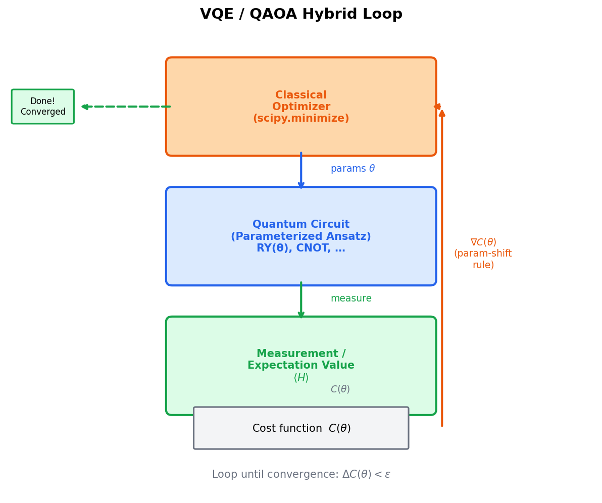
Source: mortalapps.com- Hybrid classical-quantum workflows combine classical CPUs for optimization and quantum QPUs for state preparation and measurement.
- The Variational Quantum Eigensolver (VQE) and QAOA are the leading hybrid algorithms for near-term NISQ-era hardware.
- The
Parameterclass in Qiskit allows you to define gate angles as symbolic variables, enabling dynamic, tunable circuits. - The
Estimatorprimitive is used in hybrid workflows to calculate the expectation value of physical observables. - Classical optimizers (like SciPy's COBYLA or SPSA) iteratively adjust quantum parameters to minimize a cost function.
- Using parameterized circuits and parameter binding avoids the need to rebuild and transpile circuits during each iteration.
Why This Matters
In the NISQ era, quantum computers are not standalone processors; they operate as co-processors alongside classical supercomputers. This architecture is known as a hybrid classical-quantum workflow. In a hybrid workflow, a classical computer manages the overall program flow, handles data processing, and runs optimization algorithms, while a quantum computer is used as an accelerator to execute specific, highly specialized tasks, such as calculating the expectation value of a complex quantum state.
This hybrid approach is the foundation of the most promising near-term quantum algorithms, including the Variational Quantum Eigensolver (VQE) for chemistry and the Quantum Approximate Optimization Algorithm (QAOA) for logistics. Programming these workflows requires building parameterized quantum circuits (where gate angles are represented by classical variables) and setting up iterative optimization loops that update these parameters based on quantum measurement results.
In this topic, you will master the mechanics of hybrid quantum programming in Qiskit 1.x. You will learn how to use the Parameter class to build dynamic, tunable circuits, set up an iterative optimization loop using classical libraries like SciPy, and use the Estimator primitive to calculate expectation values. You will write the complete code for a simplified variational algorithm and understand how classical and quantum processors communicate in real-time.
Core Intuition
Think of a hybrid classical-quantum workflow like a high-tech archery training system. The archer is the quantum computer, and the coach is the classical computer. The archer's bow has adjustable sights (the parameterized gates), which can be tuned to different angles (the classical parameters $\theta$).
The training session proceeds in a loop. First, the coach sets the sights to a specific angle and tells the archer to shoot 1000 arrows (run 1000 shots). The archer shoots, and the target sensors record where the arrows landed (the measurement counts). The coach analyzes the target data, calculates the average distance from the bullseye (the expectation value), and uses their classical brain (the optimization algorithm) to calculate a better sight angle.
The coach adjusts the sights to the new angle, and the archer shoots again. This loop repeats dozens of times. Neither the coach nor the archer could achieve perfection alone: the archer has the physical power to shoot the arrows (execute quantum states), but lacks the analytical capability to calculate the optimal adjustments; the coach has the analytical capability, but lacks the physical strength to shoot. Together, they quickly converge on the perfect shot.
Visualization
Technical Explanation
The core mathematical objective of a variational quantum algorithm is to find the minimum eigenvalue of a Hamiltonian operator $H$ (which represents the energy of a physical system). According to the variational principle, the expectation value of $H$ for any parameterized trial state $\lvert \psi(\theta) \rangle$ is always greater than or equal to the ground state energy $E_0$:
$$\langle H \rangle_{\theta} = \langle \psi(\theta) \lvert H \lvert \psi(\theta) \rangle \ge E_0$$
To find $E_0$, we use a classical optimizer to minimize $\langle H \rangle_{\theta}$ by iteratively updating the parameters $\theta$. In Qiskit 1.x, this workflow is driven by the Estimator primitive, which calculates expectation values directly, and the Parameter class, which allows us to define gate angles as symbolic variables.
Here is a complete, runnable Qiskit 1.x program that implements a simplified 1-qubit variational loop to find the ground state of a Pauli-Z operator:
import numpy as np
from scipy.optimize import minimize
from qiskit import QuantumCircuit
from qiskit.circuit import Parameter
from qiskit.primitives import StatevectorEstimator
from qiskit.quantum_info import SparsePauliOp

# Step 1: Define a parameterized circuit (Ansatz)
theta = Parameter('theta')
qc = QuantumCircuit(1)
qc.rx(theta, 0) # Parameterized rotation around X-axis

# Step 2: Define the observable (Hamiltonian)
# We want to find the ground state of the Pauli-Z operator
observable = SparsePauliOp('Z')

# Step 3: Instantiate the Estimator primitive
estimator = StatevectorEstimator()

# Step 4: Define the cost function for the classical optimizer
def cost_function(params):
    # params is a list of float values passed by the optimizer
    # We bind the parameter value to the circuit
    pub = (qc, observable, [params[0]])
    job = estimator.run([pub])
    result = job.result()
    # Retrieve the expectation value (energy)
    energy = result[0].data.evs
    return float(energy)

# Step 5: Run the classical optimization loop
# We start with an initial guess of theta = 0.0
initial_guess = [0.0]
print("Starting classical optimization loop...")

res = minimize(cost_function, initial_guess, method='COBYLA')

print("\nOptimization Completed!")
print(f"Optimal Parameter (theta): {res.x[0]:.4f} radians")
print(f"Minimum Expectation Value (Energy): {res.fun:.4f}")
print(f"Theoretical Minimum: -1.0000")
In this code, StatevectorEstimator is a local, noiseless primitive. The cost_function binds the classical parameter value params[0] to the symbolic Parameter('theta') in the circuit, submits it to the estimator, and returns the expectation value. The SciPy minimize function uses the COBYLA algorithm to iteratively adjust theta until the expectation value reaches its minimum value of -1.0 (which corresponds to the state $\lvert 1 \rangle$, the ground state of the $Z$ operator).
Key Takeaways
Parameter class in Qiskit allows you to define gate angles as symbolic variables, enabling dynamic, tunable circuits.Estimator primitive is used in hybrid workflows to calculate the expectation value of physical observables.